Demo the app here!
Problem Description
Just as humans have evolved into different species, birds have grown alongside them over millions of years. Adapting to changing environments and becoming one of the most diverse groups of animals on the planet, there are over 5,000 different species of birds. The goal of this project is to train a machine learning model that can accurately predict the species of a birds based on its features present in an image. Through this, I am hoping to make these majestic flying creatures seem a bit more familiar.
Previous Work
A lot of this project is based upon existing machine learning frameworks such as PyTorch. PyTorch’s flexibility and ease of use makes it a great entry way into building and training many different types of neural network architectures, whether it be convolutional or recurrent neural networks. As for the scope of this project, I found the CNN models that PyTorch provides more than adequate for the purposes of this project.
ResNet, short for Residual Network, is a deep neural network architure that was developed and described by researches at Microsoft Research. One of the key innovations of the architecture is the use of residual connections, allowing information to be directly passed from one layer to another and bypassing intermediate layers. In very deep networks like ResNet, the output of early layers can become too small to be meaningful later on in deeper layers. ResNet’s innovation helps solve this problem by allowing the network to learn more easily in these deeper layers.
EfficientNetV2 is another family of deep neural networks that is an extension of the original EfficientNet architecture. It was introduced and developed by researchers at Google. Just as the name implies, this architecture is able to achieve state-of-the-art performance on tasks such as image classification, all while maintaining great accuracy. EfficientNetV2 ranges from different models: from the small and efficient EfficientNetV2-S to the larger and more powerful EfficientNetV2-L.
Datasets
The dataset used was provided to us by the CSE 455 staff through a Kaggle competition. This dataset contained a training set of over 37,000 images of birds, spanning 555 species. Another 10,000 images are provided to evaluate the model and perform predictions to be submitted on Kaggle. Each training image has its filename and corresponding species numerical ID labeled on a ‘labels.csv’ file. Similarly, each image in the testing set also has its filename in a ‘sample.csv’ file, but with the numerical ID defaulted to 403 for us to change.
Approach
PyTorch has a great tutorial on transfer learning which this project can be attributed to.
Importing Data
Getting the dataset to be in a usuable format proved to be a problem in of itself. I needed a way to split the dataset: one part for training and another for validation. This is to help evaluate the network as its training. I created a BirdsDataset class that inherited the Dataset class so that we could make Dataloaders for the data. I made another wrapper Dataset class to help facilitate applying different transformations to the training data and validation data.
class BirdsDataset(Dataset):
    def __init__(self, csv_file, root_dir, transform=None):
        self.annotations = pd.read_csv(csv_file)
        self.root_dir = root_dir
        self.transform = transform

    def __len__(self):
        return len(self.annotations)

    def __getitem__(self, index):
        img_path = os.path.join(self.root_dir, str(self.annotations.iloc[index, 1]), self.annotations.iloc[index, 0])

        image = Image.open(img_path)
        image = image.convert("RGB") # some photos have the alpha channel

        y_label = torch.tensor(int(self.annotations.iloc[index, 1]))

        if self.transform:
            image = self.transform(image)

        return (image, y_label)

class SplitDataset(Dataset):
    def __init__(self, subset, transform=None):
        self.subset = subset
        self.transform = transform

    def __getitem__(self, index):
        x, y = self.subset[index]
        if self.transform:
            x = self.transform(x)
        return x, y

    def __len__(self):
        return len(self.subset)
To refrain from relying on PyTorch too much and to keep things novel, I also made a Python script to resize all of the images in the dataset. I employed the use of the CV framework we implemented for class. It uses nearest neighbor resizing and interpolation. This script took a little over a day to run for the training images and just a few hours for the test images.
from uwimg import *
import os

f = make_box_filter(7)
for dirpath, subdirs, files in os.walk('/mnt/c/Users/rsslr/Documents/455/birds/train'):
    for file in files:
        im = load_image(str(os.path.join(dirpath, file)))
        blur = convolve_image(im, f, 1)
        resized = nn_resize(blur, 224, 224)
        save_image(resized, str(file)[:-4])

        # cleanup
        free_image(im)
        free_image(blur)
        free_image(resized)

free_image(f)
At this point, we can start declaring our Dataloaders and applying necessary transformations for our neural network. One of the key transformations is normalization. The models I used were pretrained on ImageNet1k. As such, we normalize around the mean and stddev of the ImageNet dataset to keep things consistent.
train_transform = transforms.Compose([
    transforms.RandomCrop(224, padding=16, padding_mode='edge'),
    transforms.RandomHorizontalFlip(),
    transforms.ToTensor(),
    transforms.Normalize(mean=[0.485, 0.456, 0.406], std=[0.229, 0.224, 0.225])
])

test_transform = transforms.Compose([
    transforms.ToTensor(),
    transforms.Normalize(mean=[0.485, 0.456, 0.406], std=[0.229, 0.224, 0.225])
])

dataset = BirdsDataset(csv_file='/workspace/birds/labels.csv',
                       root_dir='/workspace/birds-resized/train',
                       transform=None)

train_subset, test_subset = torch.utils.data.random_split(dataset, [33562, 5000])

train_set = SplitDataset(train_subset, transform=train_transform)
test_set = SplitDataset(test_subset, transform=test_transform)

train_loader = DataLoader(dataset=train_set, batch_size=batch_size, shuffle=True)
test_loader = DataLoader(dataset=test_set, batch_size=batch_size, shuffle=True)

dataloaders = {'train': train_loader, 'val': test_loader}
dataset_sizes = {'train': len(train_loader.dataset), 'val': len(test_loader.dataset)}
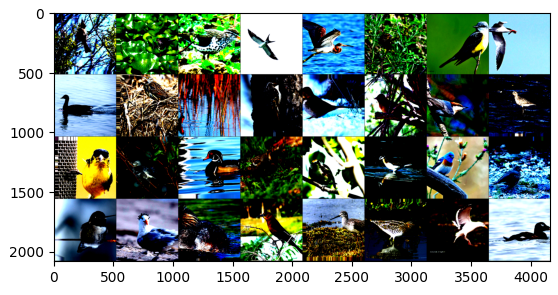
At this point, we can now view our imported data. Here is a sample batch of 32 images. Notice the unusual colors which are a product of normalization.
Defining the Model
For this project, I employed the use of two machine learning architectures: ResNet152 and EfficientNetV2-L.
model = torchvision.models.resnet152(weights='ResNet152_Weights.DEFAULT').to(device)
# OR
model = torchvision.models.efficientnet_v2_l(weights='EfficientNet_V2_L_Weights.DEFAULT').to(device)
In order for these models to work with our dataset though, we have to replace the last layer. Since these models were pretrained on ImageNet1k, they are set to have 1000 output features by default. Since our dataset contains 555 different species of birds, we want to set the output features to be 555 instead.
# The following is for EfficientNet.
# ResNet is a bit different but they're generally the same process-wise.
num_features = model.classifier[1].in_features
model.classifier[1] = nn.Linear(num_features, 555) # Add our layer with 555 outputs
Training!
I used the following training function. It’s adapted from the PyTorch transfer learning tutorial, but it has the same general functionality as the one provided to us from class tutorials.
def train_model(model, criterion, optimizer, scheduler, num_epochs=10):
    since = time.time()

    best_model_wts = copy.deepcopy(model.state_dict())
    best_acc = 0.0

    for epoch in range(num_epochs):
        print(f'Epoch {epoch}/{num_epochs - 1}')
        print('-' * 10)

        # Each epoch has a training and validation phase
        for phase in ['train', 'val']:
            if phase == 'train':
                model.train()  # Set model to training mode
            else:
                model.eval()   # Set model to evaluate mode

            running_loss = 0.0
            running_corrects = 0

            # Iterate over data.
            for inputs, labels in dataloaders[phase]:
                inputs = inputs.to(device)
                labels = labels.to(device)

                # zero the parameter gradients
                optimizer.zero_grad()

                # forward
                # track history if only in train
                with torch.set_grad_enabled(phase == 'train'):
                    outputs = model(inputs.float())
                    _, preds = torch.max(outputs, 1)
                    loss = criterion(outputs, labels)

                    # backward + optimize only if in training phase
                    if phase == 'train':
                        loss.backward()
                        optimizer.step()

                # statistics
                running_loss += loss.item() * inputs.size(0)
                running_corrects += torch.sum(preds == labels.data)
            if phase == 'train':
                scheduler.step()

            epoch_loss = running_loss / dataset_sizes[phase]
            epoch_acc = running_corrects.double() / dataset_sizes[phase]

            print(f'{phase} Loss: {epoch_loss:.4f} Acc: {epoch_acc:.4f}')

            # deep copy the model
            if phase == 'val' and epoch_acc > best_acc:
                best_acc = epoch_acc
                best_model_wts = copy.deepcopy(model.state_dict())

        print()

    time_elapsed = time.time() - since
    print(f'Training complete in {time_elapsed // 60:.0f}m {time_elapsed % 60:.0f}s')
    print(f'Best val Acc: {best_acc:4f}')

    # load best model weights
    model.load_state_dict(best_model_wts)
    return model
We can now start tweaking hyperparameters and defining things like a loss function and scheduler to facilitate training.
The optimizer implements a stochastic gradient descent optimazation algorithm. This aids in minimization of the loss function. We then have our loss function which is responsible for measuring how well the model’s predictions match the true values or labels of the training data. Lastly, we have our scheduler which is responsible for learning rate decay.
# Hyperparameters
# These were actually defined before we made the dataloaders,
# but I chose to add it here instead for readability.
in_channel = 3
num_classes = 555
learning_rate = 1e-3
batch_size = 32
num_epochs = 15
# optimizer
optimizer = optim.SGD(model.parameters(), lr=0.001, momentum=0.9)

# loss function
criterion = nn.CrossEntropyLoss()

# Decay LR by a factor of 0.1 every 7 epochs
exp_lr_scheduler = lr_scheduler.StepLR(optimizer, step_size=7, gamma=0.1)

# Start training!
model.train()
model = model.to(device)
model = train_model(model, criterion, optimizer,
                    exp_lr_scheduler, num_epochs=num_epochs)
Evaluating the Model
After the lengthy process of training, we can now start to evaluate our model. I used the same implementation for importing the training data for the test data. However, since these images don’t have an ID/label, I decided to label them with their corresponding index in the ‘sample.csv’ file. This will aid in making the final .csv for my predictions.
class TestDataset(Dataset):
    def __init__(self, csv_file, root_dir, transform=None):
        self.annotations = pd.read_csv(csv_file)
        self.root_dir = root_dir
        self.transform = transform

    def __len__(self):
        return len(self.annotations)

    def __getitem__(self, index):
        img_path = os.path.join(self.root_dir, str(self.annotations.iloc[index, 0])[5:])

        image = Image.open(img_path)
        image = image.convert("RGB") # some photos have the alpha channel

        y_label = torch.tensor(int(index))

        if self.transform:
            image = self.transform(image)

        return (image, y_label)

test_dataset = TestDataset(csv_file='/workspace/birds/sample.csv',
                       root_dir='/workspace/birds-resized/test',
                       transform=test_transform)

testing_loader = DataLoader(dataset=test_dataset, batch_size=batch_size, shuffle=False)
I set the model to evalutation mode so that it wouldn’t modify the weights when going through the data. The way the following code works is that it concatenates the label and best prediction to a Pandas DataFrame. As I’ve discussed before, the label is just the index of the corresponding image in the ‘sample.csv’ file. Then, to find the model’s best prediction for that image, we get the output’s argmax, which is just the index of the maximum value of all the elements in the input. For example, if there 555 elements and the best prediction was 0.99 at index 305, then argmax would return 305. This translates to species number 305.
df = pd.DataFrame([], [], columns=['label', 'pred'])
model.eval()
with torch.no_grad():
    for inputs, labels in testing_loader:
        inputs = inputs.to(device)
        labels = labels.to(device)

        outputs = model(inputs)
        pred = torch.argmax(outputs, 1)

        df2 = pd.DataFrame({'label': labels.cpu().numpy(), 'pred': pred.cpu().numpy()})
        df = pd.concat([df, df2], ignore_index=True)
Output:

     label pred
0        0  305
1        1  227
2        2   70
3        3  362
4        4   40
...    ...  ...
9995  9995  368
9996  9996  218
9997  9997   42
9998  9998   36
9999  9999  215

[10000 rows x 2 columns]
We’re nearly there! I then made another DataFrame to hold the final predictions. For the ‘path’ column, I took each path from ‘sample.csv’. As for the ‘class’ column, I used the corresponding ‘pred’ column from the DataFrame we created earlier.
test_csv = pd.read_csv("/workspace/birds/sample.csv")
res_csv = pd.DataFrame(columns=['path', 'class'])
for i in range(10000):
    new_row = pd.DataFrame({'path': [test_csv.iloc[i, 0]], 'class': [df.iloc[i, 1]]})
    res_csv = pd.concat([res_csv, new_row], ignore_index=True)
                                           path class
0     test/ccd7fe22b2214123aa5c7501653741e8.jpg   305
1     test/ae8d11baa5104860809d79ff626f7286.jpg   227
2     test/374ff1843b4c4b32b8f4145ae17bace0.jpg    70
3     test/df7f4ed304f6496c9dbf6350552b4858.jpg   362
4     test/ba883a3b5b34446093dc98889b957258.jpg    40
...                                         ...   ...
9995  test/8e9ac4ac8d2940b182eb4f0e29e263b7.jpg   368
9996  test/08ddc93924674259b7a318693369bd86.jpg   218
9997  test/0f6d51c0a36b4251be04d3aa83bb4b3d.jpg    42
9998  test/0e9d318a8738401090060740ef5182ea.jpg    36
9999  test/852dbbe3a24841979abb7d31e8823897.jpg   215

[10000 rows x 2 columns]
We now have our results and can export it to submit!
compression_opts = dict(method='zip',
                        archive_name='out.csv')
res_csv.to_csv('out.zip', index=False,
          compression=compression_opts)
Contents of out.csv:

path,class
test/ccd7fe22b2214123aa5c7501653741e8.jpg,305
test/ae8d11baa5104860809d79ff626f7286.jpg,227
test/374ff1843b4c4b32b8f4145ae17bace0.jpg,70
test/df7f4ed304f6496c9dbf6350552b4858.jpg,362
test/ba883a3b5b34446093dc98889b957258.jpg,40
...
Results
ResNet152
The first model I trained was ResNet152. The hyperparmeters I used for this architecture were the following: 25 epochs, a step size of 10 on the scheduler, a learning rate of 1e-3, and a batch size of 64.
Epoch 0/24
----------
train Loss: 6.0899 Acc: 0.0472
val Loss: 5.5890 Acc: 0.1330

Epoch 1/24
----------
train Loss: 4.5204 Acc: 0.2110
val Loss: 3.3127 Acc: 0.3230

Epoch 2/24
----------
train Loss: 2.7643 Acc: 0.4180
val Loss: 2.0953 Acc: 0.5030

Epoch 3/24
----------
train Loss: 1.8562 Acc: 0.5754
val Loss: 1.4755 Acc: 0.6320

Epoch 4/24
----------
train Loss: 1.3783 Acc: 0.6693
val Loss: 1.1806 Acc: 0.6958

Epoch 5/24
----------
train Loss: 1.0942 Acc: 0.7289
val Loss: 0.9961 Acc: 0.7298

Epoch 6/24
----------
train Loss: 0.8997 Acc: 0.7702
val Loss: 0.8827 Acc: 0.7588

Epoch 7/24
----------
train Loss: 0.7555 Acc: 0.8046
val Loss: 0.8016 Acc: 0.7700

Epoch 8/24
----------
train Loss: 0.6539 Acc: 0.8310
val Loss: 0.7430 Acc: 0.7892

Epoch 9/24
----------
train Loss: 0.5682 Acc: 0.8526
val Loss: 0.6991 Acc: 0.7938

Epoch 10/24
----------
train Loss: 0.4839 Acc: 0.8810
val Loss: 0.6811 Acc: 0.8012

Epoch 11/24
----------
train Loss: 0.4703 Acc: 0.8889
val Loss: 0.6755 Acc: 0.8066

Epoch 12/24
----------
train Loss: 0.4539 Acc: 0.8895
val Loss: 0.6724 Acc: 0.8072

Epoch 13/24
----------
train Loss: 0.4482 Acc: 0.8929
val Loss: 0.6719 Acc: 0.8106

Epoch 14/24
----------
train Loss: 0.4435 Acc: 0.8943
val Loss: 0.6619 Acc: 0.8074

Epoch 15/24
----------
train Loss: 0.4324 Acc: 0.8974
val Loss: 0.6603 Acc: 0.8072

Epoch 16/24
----------
train Loss: 0.4297 Acc: 0.8984
val Loss: 0.6578 Acc: 0.8142

Epoch 17/24
----------
train Loss: 0.4257 Acc: 0.8993
val Loss: 0.6531 Acc: 0.8108

Epoch 18/24
----------
train Loss: 0.4164 Acc: 0.8994
val Loss: 0.6513 Acc: 0.8120

Epoch 19/24
----------
train Loss: 0.4112 Acc: 0.9035
val Loss: 0.6456 Acc: 0.8138

Epoch 20/24
----------
train Loss: 0.4023 Acc: 0.9057
val Loss: 0.6522 Acc: 0.8110

Epoch 21/24
----------
train Loss: 0.4059 Acc: 0.9034
val Loss: 0.6478 Acc: 0.8124

Epoch 22/24
----------
train Loss: 0.4036 Acc: 0.9053
val Loss: 0.6468 Acc: 0.8140

Epoch 23/24
----------
train Loss: 0.4023 Acc: 0.9050
val Loss: 0.6475 Acc: 0.8182

Epoch 24/24
----------
train Loss: 0.4036 Acc: 0.9063
val Loss: 0.6462 Acc: 0.8164

Training complete in 255m 53s
Best val Acc: 0.818200
This gave me some pretty good results with a final validation accuracy of 0.818200. We can see the model start to converge around epoch 10, as validation loss stays stagnant while training loss continues to increase ever so slightly with every epoch. This may indicate some overfitting to the training data.
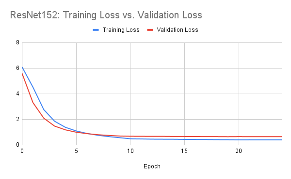
Evaluation using this model gave me a public score of 0.827 on the Kaggle competition.

EfficientNetV2-L
The second model I trained was EfficientNetV2-L. The hyperparameters I used for this architecture were the following: 15 epochs, a step size of 7 on the scheduler, a learning rate of 1e-3, and a batch size of 32.
Epoch 0/14
----------
train Loss: 5.1449 Acc: 0.1331
val Loss: 2.8316 Acc: 0.4956

Epoch 1/14
----------
train Loss: 2.2729 Acc: 0.5194
val Loss: 1.1910 Acc: 0.7328

Epoch 2/14
----------
train Loss: 1.3353 Acc: 0.6832
val Loss: 0.7842 Acc: 0.7998

Epoch 3/14
----------
train Loss: 0.9672 Acc: 0.7576
val Loss: 0.6170 Acc: 0.8362

Epoch 4/14
----------
train Loss: 0.7723 Acc: 0.8015
val Loss: 0.5320 Acc: 0.8520

Epoch 5/14
----------
train Loss: 0.6494 Acc: 0.8297
val Loss: 0.4755 Acc: 0.8634

Epoch 6/14
----------
train Loss: 0.5550 Acc: 0.8500
val Loss: 0.4409 Acc: 0.8702

Epoch 7/14
----------
train Loss: 0.4754 Acc: 0.8761
val Loss: 0.4262 Acc: 0.8748

Epoch 8/14
----------
train Loss: 0.4611 Acc: 0.8819
val Loss: 0.4131 Acc: 0.8796

Epoch 9/14
----------
train Loss: 0.4570 Acc: 0.8821
val Loss: 0.4079 Acc: 0.8792

Epoch 10/14
----------
train Loss: 0.4386 Acc: 0.8864
val Loss: 0.4115 Acc: 0.8824

Epoch 11/14
----------
train Loss: 0.4391 Acc: 0.8869
val Loss: 0.4001 Acc: 0.8822

Epoch 12/14
----------
train Loss: 0.4296 Acc: 0.8890
val Loss: 0.3984 Acc: 0.8846

Epoch 13/14
----------
---------------------------------------------------------------------------
KeyboardInterrupt
...
These results were far much better than ResNet152. The trained EffNetV2 model had a final validation accuracy of 0.8846, which is a 0.0664 difference over ResNet! We can see that the model starts to converge around epoch 9-10, where training loss and validations seem to stagnate. Based on this data, it seems that the network is learning well and isn’t overfitting to the training data as much as the loss levels are around the same.
The interesting part, though, was that EfficientNetV2-L took just as long to train 13 epochs as it did to train 25 epochs with ResNet. Doing a little research, it seems that ResNet152 has 60.2 million parameters while EfficientNetV2-L has 118.5 million parameters. Looking at the Medium variant of EfficientNetV2, it’s reported to have 54.1 million parameters. If we were to use that model instead, I think the performance would be as comparable to ResNet.
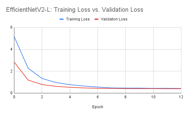
Evaluation using this model gave me a public score of 0.88950 on the Kaggle competition. As of 3/14/2023, this model currently sits atop the leaderboards!


Discussion
Problems encountered
One of the first problems I encountered was getting the dataset to be in a usable state. Loading the data was straightforward, but during training, the notebook kernel would sometimes crash because of a tensor shape error. It took me some time to diagnose this, but it turns out some of the images had a fourth alpha channel. Splicing that channel off took care of the problem. Another problem I had with the data was splitting it into two parts: training and validation. Since we aren’t supplied with a validation set, I decided to use 5000 random images from the training set instead. However, using just the random_split() function wasn’t adequate enough because it wouldn’t allow me to apply different transformations to that validation set; it would use the training transformations for both. Thus, I made another wrapper Dataset class to help facilitate applying different transformations to the split dataset.
Another problem I encountered was resource constraints. Kaggle allots you 30 hours of GPU time per week. I ended up exceeding this time limit experimenting with different models and parameters, prompting me to move to Google Colab. However, Colab wasn’t meant for long-term computing tasks like machine learning model training, so I was quickly limited there too. I ended up spending $10 renting an RTX 4090 on vast.ai to accelerate training times. Using a 4090 was much faster than the free tier GPUs on Kaggle and Colab.
Next steps
One of the things I proposed to do for this project was real-time object-detection and classification using video input. I wanted to try out frameworks like YOLO, but like all things in life, time has been a major constraint. And since object-detection frameworks like YOLO require drawing a bounding box around objects, doing this with over 40,000 images was too daunting of a task. This is definitely something I would like to dive into when I do have the time, though. Sites like Roboflow use machine learning to make this bounding box operation streamlined, which is especially useful for larger datasets.
Something I also want to experiment with is data parallelism using multiple GPUs. When I was training using an RTX 4090 on vast.ai, I noticed the options to use up to 8+ GPUs. This made me curious about how much multiple GPUs would accelerate training time, especially with models like EfficientNetV2-L which has more than 100 million parameters.
Lastly, I also would like to test even deeper netowrk architectures like VisionTransofrmer which has 633.5 million parameters and able to achieve 98.694 top 5 accuracy on ImageNet1k. I tried to use this network model, but I kept running into VRAM errors, even with batch sizes as low as 8 or 4. If I had the resources, I would defintely like to test this.
Novelty
Some of the things I think made my approch novel was the use of different and deeper models. I noticed that in tutorial, architectures like ResNet18 were used. These are great for general use cases, but for bigger datasets like the one for this project, I was aiming to have one of the best model performances. I also thought that my short Python script for image resizing kept things fresh. Even though doing this augmentation would be much faster using PyTorch, I had the time to spare. Lastly, I think that my bird classifier webapp gave a sense of practicality as something similar could be used for other classification tasks.